Instrumental variables I & II

Lecture videos
Videos for each section of the lecture and the R demonstration are available at this YouTube playlist.
- Introduction
- Endogeneity & exogeneity
- Instruments
- Using instruments
- IV with R (forthcoming)
- Treatment effects & compliance (forthcoming)
You can also watch the playlist (and skip around to different sections) here:
R stuff
Download all the R stuff you need to play along at home: week-12.zip. You can also open an RStudio.cloud project with everything ready to go.
Get data for examples
Download these CSV files and put them in a folder named data in a new RStudio project:
IV/2SLS examples
library(tidyverse)   # For ggplot, %>%, and friends
library(broom)       # For converting models to data frames
library(huxtable)    # For side-by-side regression tables
library(wooldridge)  # For some econometrics datasets
library(estimatr)    # For iv_robust
Education, wages, and parent education (fake data)
ed_fake <- read_csv("data/father_education.csv")We’re interested in the perennial econometrics question of whether an extra year of education causes increased wages. In this example we use simulated/fake data that includes the following variables:
| Variable name | Description |
|---|---|
wage |
Weekly wage |
educ |
Years of education |
ability |
Magical column that measures your ability to work and go to school (omitted variable) |
fathereduc |
Years of education for father |
If we could actually measure ability, we could estimate this model, which closes the confounding backdoor posed by ability and isolates just the effect of education on wages:
model_perfect <- lm(wage ~ educ + ability, data = ed_fake)
tidy(model_perfect)| term | estimate | std.error | statistic | p.value |
|---|---|---|---|---|
| (Intercept) | -80.263 | 5.659 | -14.2 | 0 |
| educ | 9.242 | 0.343 | 27.0 | 0 |
| ability | 0.258 | 0.007 | 35.9 | 0 |
However, in real life we don’t have ability, so we’re stuck with a naive model:
model_naive <- lm(wage ~ educ, data = ed_fake)
tidy(model_naive)| term | estimate | std.error | statistic | p.value |
|---|---|---|---|---|
| (Intercept) | -53.1 | 8.492 | -6.25 | 0 |
| educ | 12.2 | 0.503 | 24.32 | 0 |
The naive model overestimates the effect of education on wages (12.2 vs. 9.24) because of omitted variable bias. Education suffers from endogeneity—there are things in the model (like ability, hidden in the error term) that are correlated with it. Any estimate we calculate will be wrong and biased because of selection effects or omitted variable bias (all different names for endogeneity).
To fix the endogeneity problem, we can use an instrument to remove the endogeneity from education and instead use a special exogeneity-only version of education. Perhaps someone’s father’s education can be an instrument for education.
To be a valid instrument, it must meet three criteria:
- Relevance: Instrument is correlated with policy variable
- Exclusion: Instrument is correlated with outcome only through the policy variable
- Exogeneity: Instrument isn’t correlated with anything else in the model (i.e. omitted variables)
We can first test relevance by making a scatterplot and running a model of policy ~ instrument:
ggplot(ed_fake, aes(x = fathereduc, y = educ)) +
  geom_point() +
  geom_smooth(method = "lm")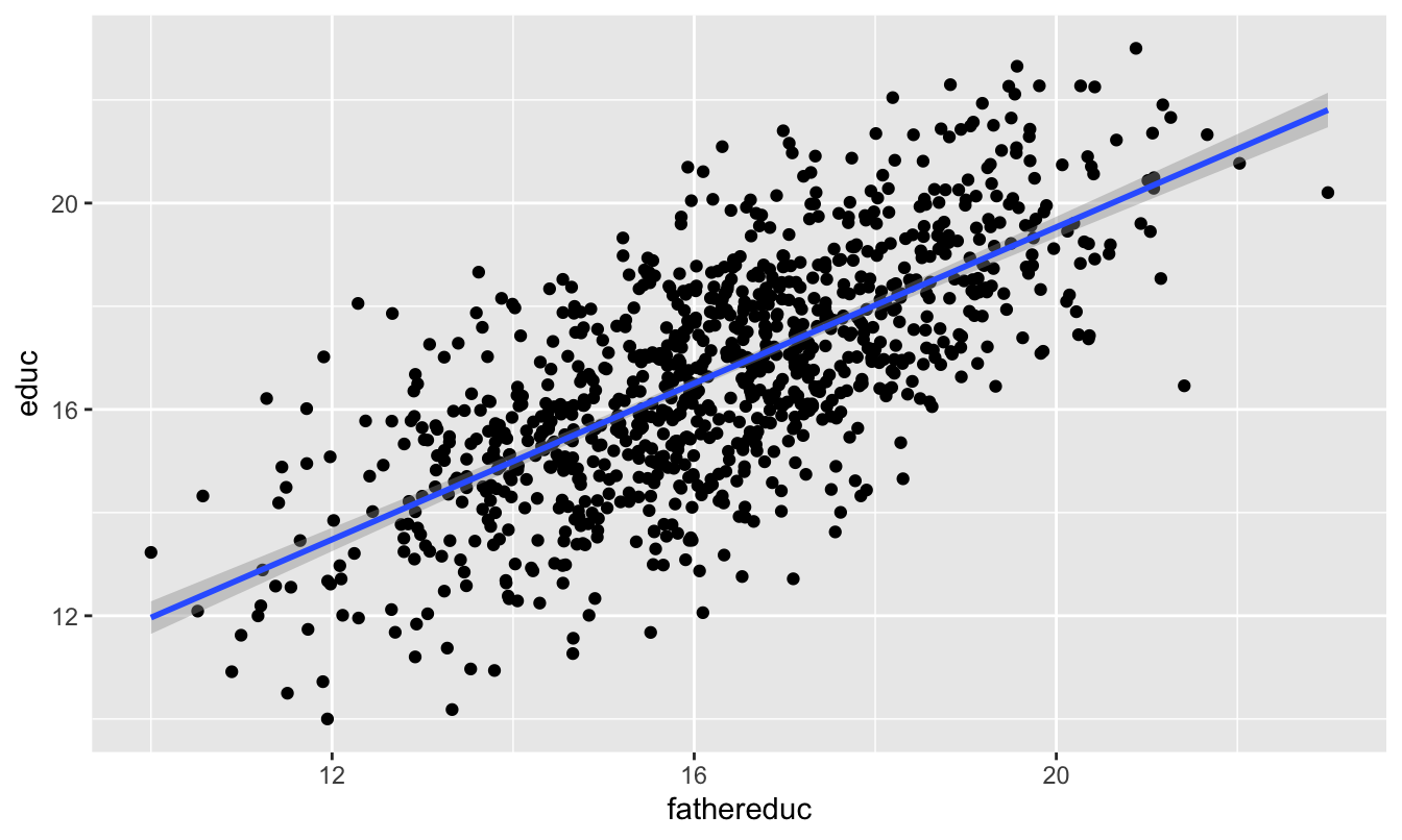
check_relevance <- lm(educ ~ fathereduc, data = ed_fake)
tidy(check_relevance)| term | estimate | std.error | statistic | p.value |
|---|---|---|---|---|
| (Intercept) | 4.396 | 0.399 | 11.0 | 0 |
| fathereduc | 0.757 | 0.024 | 31.2 | 0 |
glance(check_relevance)| r.squared | adj.r.squared | sigma | statistic | p.value | df | logLik | AIC | BIC | deviance | df.residual |
|---|---|---|---|---|---|---|---|---|---|---|
| 0.493 | 0.493 | 1.6 | 972 | 0 | 2 | -1885 | 3777 | 3791 | 2541 | 998 |
This looks pretty good! The F-statistic is definitely above 10 (it’s 972!), and there’s a significant relationship between the instrument and policy. I’d say that this is relevant.
To check for exclusion, we need to see if there’s a relationship between father’s education and wages that occurs only because of education. If we plot it, we’ll see a relationship:
ggplot(ed_fake, aes(x = fathereduc, y = wage)) +
  geom_point() +
  geom_smooth(method = "lm")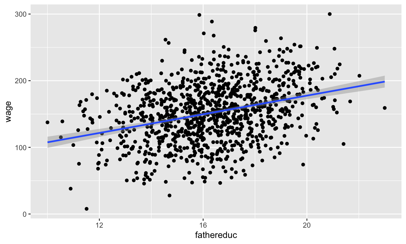
That’s to be expected, since in our model, father’s education causes education which causes wages—they should be correlated. We have to use theory to justify the idea that a father’s education increases the hourly wage only because it increases one’s education, and there’s no real statistical test for that.
There’s not really a test for exogeneity either, since there’s no way to measure other endogenous variables in the model (that’s the whole reason we’re using IVs in the first place!). Because we have the magical ability column in this fake data, we can test it. Father’s education shouldn’t be related to ability:
ggplot(ed_fake, aes(x = ability, y = fathereduc)) +
  geom_point() +
  geom_smooth(method = "lm")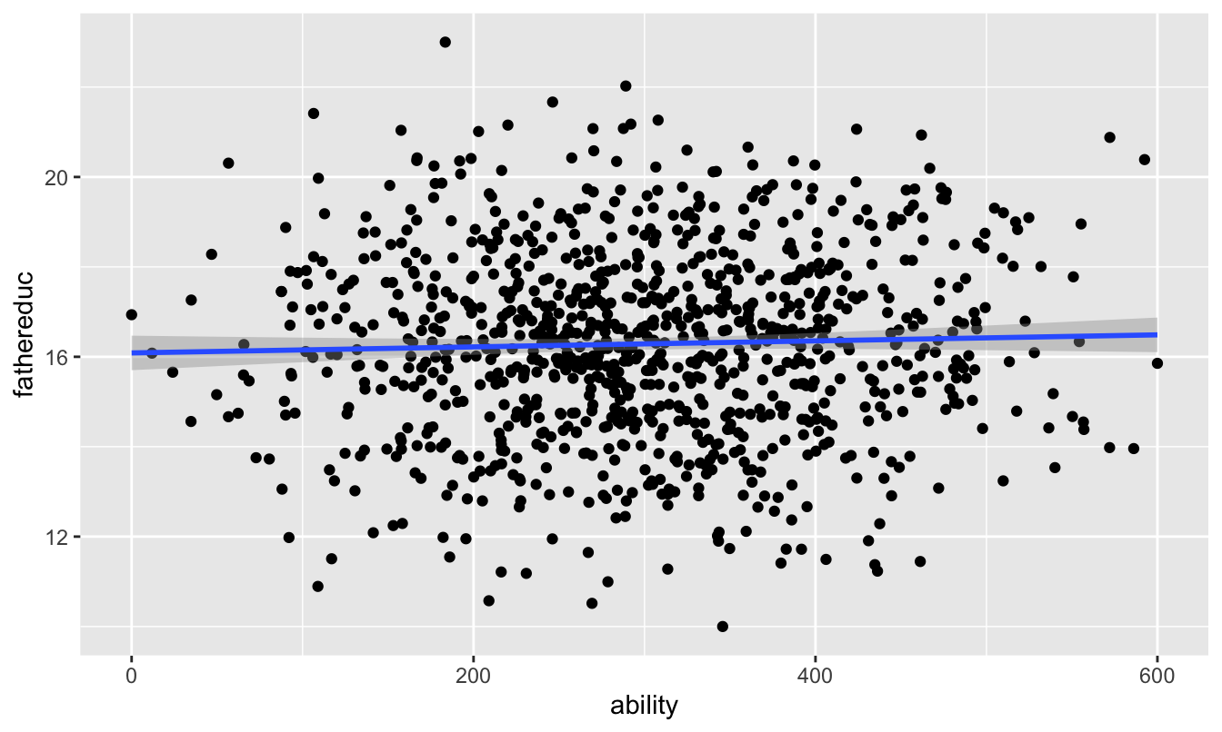
And it’s not! We can safely say that it meets the exclusion assumption.
For the last part—the exogeneity assumption—there’s no statistical test. We just have to tell a theory-based story that the number of years of education one’s father has is not correlated with anything else in the model (including any omitted variables). Good luck with that—it’s probably not a good instrument. This relates to Scott Cunningham’s argument that instruments have to be weird. According to Scott:
The reason I think this is because an instrument doesn’t belong in the structural error term and the structural error term is all the intuitive things that determine your outcome. So it must be weird, otherwise it’s probably in the error term.
Let’s just pretend that father’s education is a valid instrument and move on :)
Now we can do two-stage least squares (2SLS) regressin and use the instrument to filter out the endogenous part of education. The first stage predicts education based on the instrument (we already ran this model earlier when checking for relevance, but we’ll do it again just for fun):
first_stage <- lm(educ ~ fathereduc, data = ed_fake)Now we want to add a column of predicted education to our original dataset. The easiest way to do that is with the augment_columns() function from the broom library:
ed_fake_with_prediction <- augment_columns(first_stage, ed_fake)
head(ed_fake_with_prediction)| wage | educ | ability | fathereduc | .fitted | .se.fit | .resid | .hat | .sigma | .cooksd | .std.resid |
|---|---|---|---|---|---|---|---|---|---|---|
| 146 | 18.1 | 348 | 17.2 | 17.4 | 0.055 | 0.670 | 0.001 | 1.60 | 0.000 | 0.420 |
| 148 | 15.8 | 181 | 14.0 | 15.0 | 0.075 | 0.862 | 0.002 | 1.60 | 0.000 | 0.541 |
| 162 | 15.1 | 337 | 16.0 | 16.5 | 0.051 | -1.397 | 0.001 | 1.60 | 0.000 | -0.876 |
| 105 | 16.5 | 106 | 21.4 | 20.6 | 0.134 | -4.145 | 0.007 | 1.59 | 0.024 | -2.607 |
| 168 | 18.8 | 302 | 16.5 | 16.9 | 0.051 | 1.941 | 0.001 | 1.59 | 0.001 | 1.217 |
| 173 | 16.0 | 284 | 15.4 | 16.1 | 0.055 | -0.055 | 0.001 | 1.60 | 0.000 | -0.035 |
Note a couple of these new columns. .fitted is the fitted/predicted value of education, and it’s the version of education with endogeneity arguably removed. .resid shows how far off the prediction is from educ. The other columns don’t matter so much.
Instead of dealing with weird names like .fitted, I like to rename the fitted variable to something more understandable after I use augment_columns:
ed_fake_with_prediction <- augment_columns(first_stage, ed_fake) %>%
  rename(educ_hat = .fitted)

head(ed_fake_with_prediction)| wage | educ | ability | fathereduc | educ_hat | .se.fit | .resid | .hat | .sigma | .cooksd | .std.resid |
|---|---|---|---|---|---|---|---|---|---|---|
| 146 | 18.1 | 348 | 17.2 | 17.4 | 0.055 | 0.670 | 0.001 | 1.60 | 0.000 | 0.420 |
| 148 | 15.8 | 181 | 14.0 | 15.0 | 0.075 | 0.862 | 0.002 | 1.60 | 0.000 | 0.541 |
| 162 | 15.1 | 337 | 16.0 | 16.5 | 0.051 | -1.397 | 0.001 | 1.60 | 0.000 | -0.876 |
| 105 | 16.5 | 106 | 21.4 | 20.6 | 0.134 | -4.145 | 0.007 | 1.59 | 0.024 | -2.607 |
| 168 | 18.8 | 302 | 16.5 | 16.9 | 0.051 | 1.941 | 0.001 | 1.59 | 0.001 | 1.217 |
| 173 | 16.0 | 284 | 15.4 | 16.1 | 0.055 | -0.055 | 0.001 | 1.60 | 0.000 | -0.035 |
We can now use the new educ_hat variable in our second stage model:
second_stage <- lm(wage ~ educ_hat, data = ed_fake_with_prediction)
tidy(second_stage)| term | estimate | std.error | statistic | p.value |
|---|---|---|---|---|
| (Intercept) | -3.11 | 14.370 | -0.216 | 0.829 |
| educ_hat | 9.25 | 0.856 | 10.814 | 0.000 |
The estimate for educ_hat is arguably more accurate now because we’ve used the instrument to remove the endogenous part of education and should only have the exogenous part.
We can put all the models side-by-side to compare them:
huxreg(list("Perfect" = model_perfect, "OLS" = model_naive, "2SLS" = second_stage))| Perfect | OLS | 2SLS | |
| (Intercept) | -80.263 *** | -53.085 *** | -3.108 |
| (5.659) | (8.492) | (14.370) | |
| educ | 9.242 *** | 12.240 *** | |
| (0.343) | (0.503) | ||
| ability | 0.258 *** | ||
| (0.007) | |||
| educ_hat | 9.252 *** | ||
| (0.856) | |||
| N | 1000 | 1000 | 1000 |
| R2 | 0.726 | 0.372 | 0.105 |
| logLik | -4576.101 | -4991.572 | -5168.868 |
| AIC | 9160.202 | 9989.144 | 10343.735 |
| *** p < 0.001; ** p < 0.01; * p < 0.05. | |||
Note how the coefficient for educ_hat in the 2SLS model is basically the same as the coefficient for educ in the perfect model that accounts for ability. That’s the magic of instrumental variables!
Education, wages, and parent education (real data)
This data comes from the wage2 dataset in the wooldridge R package (and it’s real!). Wages are measured in monthly earnings in 1980 dollars.
wage2 <- read_csv("data/wage2.csv")ed_real <- wage2 %>%
rename(education = educ, education_dad = feduc, education_mom = meduc) %>%
na.omit() # Get rid of rows with missing valuesWe want to again estimate the effect of education on wages, but this time we’ll use both one’s father’s education and one’s mother’s education as instruments. Here’s the naive estimation of the relationship, which suffers from endogeneity:
model_naive <- lm(wage ~ education, data = ed_real)
tidy(model_naive)| term | estimate | std.error | statistic | p.value |
|---|---|---|---|---|
| (Intercept) | 175.2 | 92.8 | 1.89 | 0.06 |
| education | 59.5 | 6.7 | 8.88 | 0.00 |
This is wrong though! Education is endogenous to unmeasured things in the model (like ability, which lives in the error term). We can isolate the exogenous part of education with an instrument.
Before doing any 2SLS models, we want to check the validity of the instruments. Remember, for an instrument to be valid, it should meet these criteria:
- Relevance: Instrument is correlated with policy variable
- Exclusion: Instrument is correlated with outcome only through the policy variable
- Exogeneity: Instrument isn’t correlated with anything else in the model (i.e. omitted variables)
We can check for relevance by looking at the relationship between the instruments and education:
# Combine father's and mother's education into one column so we can plot both at the same time
ed_real_long <- ed_real %>%
  pivot_longer(cols = c(education_dad, education_mom),
               names_to = "instrument", values_to = "instrument_value")

ggplot(ed_real_long, aes(x = instrument_value, y = education)) +
  geom_point() +
  geom_smooth(method = "lm") +
  facet_wrap(~ instrument)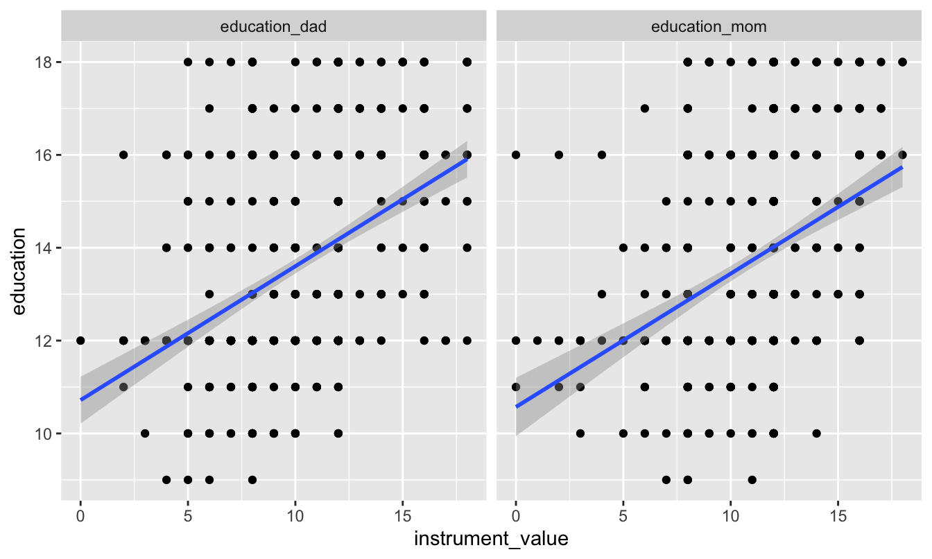
model_check_instruments <- lm(education ~ education_dad + education_mom,
                              data = ed_real)
tidy(model_check_instruments)| term | estimate | std.error | statistic | p.value |
|---|---|---|---|---|
| (Intercept) | 9.913 | 0.320 | 31.02 | 0 |
| education_dad | 0.219 | 0.029 | 7.58 | 0 |
| education_mom | 0.140 | 0.034 | 4.17 | 0 |
glance(model_check_instruments)| r.squared | adj.r.squared | sigma | statistic | p.value | df | logLik | AIC | BIC | deviance | df.residual |
|---|---|---|---|---|---|---|---|---|---|---|
| 0.202 | 0.199 | 2 | 83.3 | 0 | 3 | -1398 | 2804 | 2822 | 2632 | 660 |
There’s a clear relationship between both of the instruments and education, and the coefficients for each are signficiant. The F-statistic for the model is 83, which is higher than 10, which is a good sign of a strong instrument.
We can check for exclusion in part by looking at the relationship between the instruments and the outcome, or wages. We should see some relationship:
ggplot(ed_real_long, aes(x = instrument_value, y = wage)) +
  geom_point() +
  geom_smooth(method = "lm") +
  facet_wrap(~ instrument)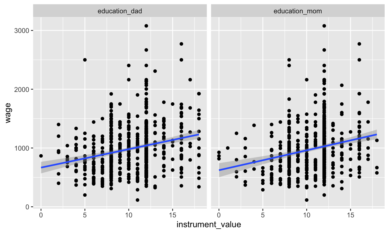
And we do! Now we just have to make the case that the only reason there’s a relationship is that parental education only influences wages through education. Good luck with that.
The last step is to prove exogeneity—that parental education is not correlated with education or wages. Good luck with that too.
Assuming that parental education is a good instrument, we can use it to remove the endogenous part of education using 2SLS. In the first stage, we predict education using our instruments:
first_stage <- lm(education ~ education_dad + education_mom, data = ed_real)We can then extract the predicted education and add it to our main dataset, renaming the .fitted variable to something more useful along the way:
ed_real_with_predicted <- augment_columns(first_stage, ed_real) %>%
  rename(education_hat = .fitted)
Finally, we can use predicted education to estimate the exogenous effect of education on wages:
second_stage <- lm(wage ~ education_hat,
                   data = ed_real_with_predicted)
tidy(second_stage)| term | estimate | std.error | statistic | p.value |
|---|---|---|---|---|
| (Intercept) | -538 | 208.2 | -2.58 | 0.01 |
| education_hat | 112 | 15.2 | 7.35 | 0.00 |
That should arguably be our actual effect! Let’s compare it to the naive model:
huxreg(list("OLS" = model_naive, "2SLS" = second_stage))| OLS | 2SLS | |
| (Intercept) | 175.160 | -537.712 * |
| (92.839) | (208.164) | |
| education | 59.452 *** | |
| (6.698) | ||
| education_hat | 111.561 *** | |
| (15.176) | ||
| N | 663 | 663 |
| R2 | 0.106 | 0.076 |
| logLik | -4885.974 | -4897.252 |
| AIC | 9777.947 | 9800.503 |
| *** p < 0.001; ** p < 0.01; * p < 0.05. | ||
The 2SLS effect is roughly twice as large and is arguably more accurate, since it has removed the endogeneity from education. An extra year of school leads to an extra $111.56 dollars a month in income (in 1980 dollars).
If you don’t want to go through the hassle of doing the two stages by hand, you can use the iv_robust() function from the estimatr package to do both stages at the same time. The second stage goes on the left side of the |, just like a normal regression. The first stage goes on the right side of the |:
model_same_time <- iv_robust(wage ~ education | education_dad + education_mom,
                             data = ed_real)
tidy(model_same_time)| term | estimate | std.error | statistic | p.value | conf.low | conf.high | df | outcome |
|---|---|---|---|---|---|---|---|---|
| (Intercept) | -538 | 214.4 | -2.51 | 0.012 | -958.8 | -117 | 661 | wage |
| education | 112 | 15.9 | 7.02 | 0.000 | 80.3 | 143 | 661 | wage |
We should get the same coefficient as the second stage, but the standard errors with iv_robust are more accurate. The only problem with iv_robust is that there’s no way to see the first stage, so if you want to check for relevancy or show the F-test or show the coefficients for the instruments, you’ll have to run a first_stage model on your own.
Models from iv_robust() also work with huxreg(). Note how the education variable isn’t renamed educ_hat in the iv_robust() version—it’s still using predicted education even if it’s not obvious
huxreg(list("OLS" = model_naive, "2SLS" = second_stage,
"2SLS iv_robust" = model_same_time))| OLS | 2SLS | 2SLS iv_robust | |
| (Intercept) | 175.160 | -537.712 * | -537.712 * |
| (92.839) | (208.164) | (214.431) | |
| education | 59.452 *** | 111.561 *** | |
| (6.698) | (15.901) | ||
| education_hat | 111.561 *** | ||
| (15.176) | |||
| N | 663 | 663 | 663 |
| R2 | 0.106 | 0.076 | 0.025 |
| logLik | -4885.974 | -4897.252 | |
| AIC | 9777.947 | 9800.503 | |
| *** p < 0.001; ** p < 0.01; * p < 0.05. | |||
Education, wages, and distance to college (real data)
For this last example we’ll estimate the effect of education on wages using a different instrument—geographic proximity to colleges. This data comes from David Card’s 1995 study where he did the same thing, and it’s available in the wooldridge library as card. You can find a description of all variables here; we’ll use these:
| Variable name | Description |
|---|---|
lwage |
Annual wage (log form) |
educ |
Years of education |
nearc4 |
Living close to college (=1) or far from college (=0) |
smsa |
Living in metropolitan area (=1) or not (=0) |
exper |
Years of experience |
expersq |
Years of experience (squared term) |
black |
Black (=1), not black (=0) |
south |
Living in the south (=1) or not (=0) |
Once again, Card wants to estimate the impact of education on wage. But to solve the ability bias, he utilizes a different instrumental variable: proximity to college. He provides arguments to support each of three main characteristics of a good instrumental variable:
- Relevancy: People who live close to a 4-year college have easier access to education at a lower costs (no commuting costs and time nor accommodation costs), so they have greater incentives to pursue education.
- Exclusion: Proximity to a college has no effect on your annual income, unless you decide to pursue further education because of the nearby college.
- Exogeneity: Individual ability does not depend on proximity to a college.
Therefore, he estimates a model where:
First stage:
\[ \widehat{\text{Educ}} = \beta_0 + \beta_1\text{nearc4} + \beta_{2-6}\text{Control variables} \]
Second stage:
\[ \text{lwage} = \beta_0 + \beta_1 \widehat{\text{Educ}} + \beta_{2-6}\text{Control variables} \]
He controls for five things: smsa66 + exper + expersq + black + south66.
We can do the same thing. IMPORTANT NOTE: When you include controls, every control variable needs to go in both stages. The only things from the first stage that don’t carry over to the second stage are the instruments—notice how nearc4 is only in the first stage, since it’s the instrument, but it’s not in the second stage. The other controls are all in both stages.
card <- read_csv("data/card.csv")# First we'll build a naive model without any instruments so we can see the bias
# in the educ coefficient
naive_model <- lm(lwage ~ educ + smsa66 + exper + expersq + black + south66,
data = card)
# Then we'll run the first stage, predicting educ with nearc4 + all the controls
first_stage <- lm(educ ~ nearc4 + smsa66 + exper + expersq + black + south66,
data = card)
# Then we'll add the fitted education values into the original dataset and
# rename the .fitted column so it's easier to work with
card <- augment_columns(first_stage, card) %>%
rename(educ_hat = .fitted)
# Finally we can run the second stage model using the predicted education from
# the first stage
second_stage <- lm(lwage ~ educ_hat + smsa66 + exper + expersq + black + south66,
data = card)
# Just for fun, we can do all of this at the same time with iv_robsust
model_2sls <- iv_robust(lwage ~ educ + smsa66 + exper + expersq + black + south66 |
nearc4 + smsa66 + exper + expersq + black + south66,
data = card)huxreg(list("OLS" = naive_model, "2SLS" = second_stage, "2SLS iv_robust" = model_2sls))| OLS | 2SLS | 2SLS iv_robust | |
| (Intercept) | 4.731 *** | 3.357 *** | 3.357 *** |
| (0.069) | (0.926) | (0.930) | |
| educ | 0.076 *** | 0.157 ** | |
| (0.004) | (0.055) | ||
| smsa66 | 0.113 *** | 0.081 ** | 0.081 ** |
| (0.015) | (0.027) | (0.027) | |
| exper | 0.085 *** | 0.118 *** | 0.118 *** |
| (0.007) | (0.023) | (0.024) | |
| expersq | -0.002 *** | -0.002 *** | -0.002 *** |
| (0.000) | (0.000) | (0.000) | |
| black | -0.177 *** | -0.104 | -0.104 * |
| (0.018) | (0.053) | (0.052) | |
| south66 | -0.096 *** | -0.064 * | -0.064 * |
| (0.016) | (0.028) | (0.028) | |
| educ_hat | 0.157 ** | ||
| (0.055) | |||
| N | 3010 | 3010 | 3010 |
| R2 | 0.269 | 0.160 | 0.143 |
| logLik | -1352.703 | -1563.264 | |
| AIC | 2721.406 | 3142.528 | |
| *** p < 0.001; ** p < 0.01; * p < 0.05. | |||
Notice how educ_hat and educ are the same in each of the 2SLS models, and they’re higher than the naive uninstrumented model. Because the outcome is log wages, we can say that an extra year of education causes a 15.7% increase in wages.
ITT and CACE
Compliance
In class we talked about the difference between the average treatment effect (ATE), or the average effect of a program for an entire population, and conditional averages treatment effects (CATE), or the average effect of a program for some segment of the population. There are all sorts of CATEs: you can find the CATE for men vs. women, for people who are treated with the program (the average treatment on the treated, or ATT or TOT), for people who are not treated with the program (the average treatment on the untreated, or ATU), and so on.
One important type of CATE is the effect of a program on just those who comply with the program. We can call this the complier average treatment effect, but the acronym would be the same as conditional average treatment effect, so we’ll call it the conditional average causal effect (CACE).
Thinking about compliance is important. You might randomly assign people to receive treatment or a program, but people might not do what you tell them. Additionally, people might do the program if assigned to do it, but they would have done it anyway. We can split the population into four types of people:
- Compliers: People who follow whatever their assignment is (if assigned to treatment, they do the program; if assigned to control, they don’t)
- Always takers: People who will receive or seek out the program regardless of assignment (if assigned to treatment, they do the program; if assigned to control, they still do the program)
- Never takers: People who will not receive or seek out the program regardless of assignment (if assigned to treatment, they don’t do the program; if assigned to control, they also don’t do it)
- Defiers: People who will do the opposite of whatever their assignment is (if assigned to treatment, they don’t do the program; if assigned to control, they do the program)
To simplify things, evaluators and econometricians assume that defiers don’t exist based on the idea of monotonicity, which means that we can assume that the effect of being assigned to treatment only increases the likelihood of participating in the program (and doesn’t make it more likely).
The tricky part about trying to find who the compliers are in a sample is that we can’t know what people would have done in the absence of treatment. If we see that someone in the experiment was assigned to be in the treatment group and they then participated in the program, they could be a complier (since they did what they were assigned to do), or they could be an always taker (they did what they were assigned to do, but they would have done it anyway). Due to the fundamental problem of causal inference, we cannot know what each person would have done in a parallel world.
We can use data from a hypothetical program to see how these three types of compliers distort our outcomes.
library(tidyverse)
library(broom)
library(estimatr)

bed_nets <- read_csv("data/bed_nets_observed.csv") %>%
  # Make "No bed net" (control) the base case
  mutate(bed_net = fct_relevel(bed_net, "No bed net"))

bed_nets_time_machine <- read_csv("data/bed_nets_time_machine.csv") %>%
  mutate(bed_net = fct_relevel(bed_net, "No bed net"))
This is what we would be able to see if we could read everyone’s minds. There are always takers who will use a bed net regardless of the program, and they’ll have higher health outcomes. However, those better outcomes are because of something endogenous—there’s something else that makes these people always pursue bed nets, and that’s likely related to health. We probably want to not consider them when looking for the program effect. There are never takers who won’t ever use a bed net, and they have worse health outcomes. Again, there’d endogeneity here—something is causing them to not use the bed nets, and it likely also causes their health level. We don’t want to look at them either.
The middle group—the compliers—are the people we want to focus on. Here we see that the program had an effect when compared to a control group.
ggplot(bed_nets_time_machine, aes(y = health, x = treatment)) +
  geom_point(aes(shape = bed_net, color = status), position = "jitter") +
  facet_wrap(~ status) +
  labs(color = "Type of person", shape = "Compliance",
       x = NULL, y = "Health status")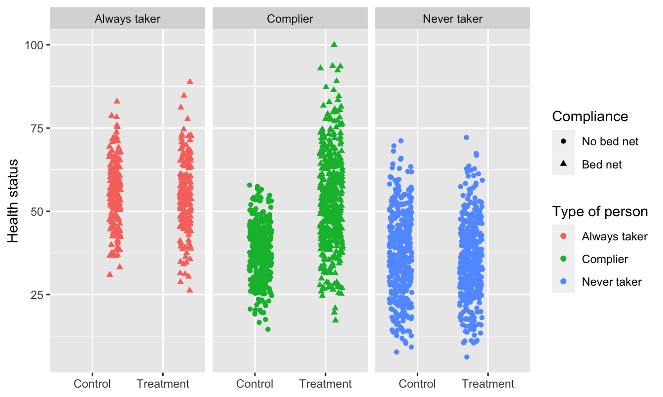
Finding compliers in actual data
This is what we actually see in the data, though. You can tell who some of the always takers are (those who used bed nets after being assigned to the control group) and who some of the never takers are (those who did not use a bed net after being assigned to the treatment group), but compliers are mixed up with the always and never takers. We have to somehow disentangle them!
ggplot(bed_nets_time_machine, aes(y = health, x = treatment)) +
  geom_point(aes(shape = bed_net, color = status), position = "jitter") +
  facet_wrap(~ bed_net) +
  labs(color = "Type of person", shape = "Compliance",
       x = NULL, y = "Health status")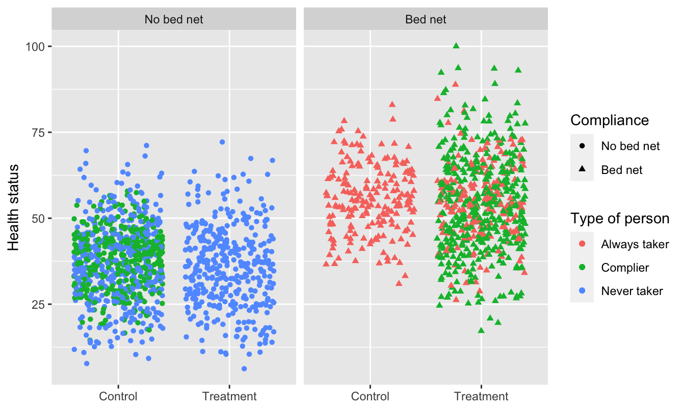
We can do this by assuming the proportion of compliers, never takers, and always takers are equally spread across treatment and control (which we can assume through the magic of randomization). If that’s the case, we can calculate the intent to treat (ITT) effect, which is the CATE of being assigned treatment (or the effect of being assigned treatment on health status, regardless of actual compliance).
The ITT is actually composed of three different causal effects: the complier average causal effect (CACE), the always taker average causal effect (ATACE), and the never taker average causal effect (NTACE). In the formula below, \(\pi\) stands for the proportion of people in each group. Formally, the ITT can be defined like this:
\[ \begin{aligned} \text{ITT} =& \pi_\text{compliers} \times (\text{T} - \text{C})_\text{compliers} + \\ &\pi_\text{always takers} \times (\text{T} - \text{C})_\text{always takers} + \\ &\pi_\text{never takers} \times (\text{T} - \text{C})_\text{never takers} \end{aligned} \]
We can simplify this to this acronymized version:
\[ \text{ITT} = \pi_\text{C} \text{CACE} + \pi_\text{A} \text{ATACE} + \pi_\text{N} \text{NTACE} \]
The number we care about the most here is the CACE, which is stuck in the middle of the equation. If we assume that assignment to treatment doesn’t make someone more likely to be an always taker or a never taker, we can set the ATACE and NTACE to zero, leaving us with just three variables to worry about: ITT, \(\pi_\text{c}\), and CACE:
\[ \begin{aligned} \text{ITT} =& \pi_\text{C} \text{CACE} + \pi_\text{A} 0 + \pi_\text{N} 0 \\ & \pi_\text{C} \text{CACE} \end{aligned} \]
We can use algebra to rearrange this formula so that we’re left with an equation that starts with CACE (since that’s the value we care about):
\[ \text{CACE} = \frac{\text{ITT}}{\pi_\text{C}} \]
If we can find the ITT and the proportion of compliers, we can find the complier average causal effect (CACE). The ITT is easy to find with a simple OLS model:
itt_model <- lm(health ~ treatment, data = bed_nets)

tidy(itt_model)| term | estimate | std.error | statistic | p.value |
|---|---|---|---|---|
| (Intercept) | 40.94 | 0.444 | 92.11 | 0 |
| treatmentTreatment | 5.99 | 0.630 | 9.51 | 0 |
ITT <- tidy(itt_model) %>%
  filter(term == "treatmentTreatment") %>%
  pull(estimate)
The ITT here is ≈6—being assigned treatment increases average health status by 5.99 health points.
The proportion of compliers is a little trickier, but doable with some algebraic trickery. Recall from the graph above that the people who were in the treatment group and who complied are a combination of always takers and compliers. This means we can say:
\[ \begin{aligned} \pi_\text{A} + \pi_\text{C} =& \text{% yes in treatment; or} \\ \pi_\text{C} =& \text{% yes in treatment} - \pi_\text{A} \end{aligned} \]
We actually know \(\pi_\text{A}\)—remember in the graph above that the people who were in the control group and who used bed nets are guaranteed to be always takers (none of them are compliers or never takers). If we assume that the proportion of always takers is the same in both treatment and control, we can use that percent here, giving us this final equation for \(\pi_\text{C}\):
\[ \pi_\text{C} = \text{% yes in treatment} - \text{% yes in control} \]
So, if we can find the percent of people assigned to treatment who used bed nets, find the percent of people assigned to control and used bed nets, and subtract the two percentages, we’ll have the proportion of compliers, or \(\pi_\text{C}\). We can do that with the data we have (61% - 19.5% = 41.5% compliers):
bed_nets %>%
  group_by(treatment, bed_net) %>%
  summarize(n = n()) %>%
  mutate(prop = n / sum(n))
## # A tibble: 4 x 4
## # Groups: treatment [2]
## treatment bed_net n prop
## <chr> <fct> <int> <dbl>
## 1 Control No bed net 808 0.805
## 2 Control Bed net 196 0.195
## 3 Treatment No bed net 388 0.390
## 4 Treatment Bed net 608 0.610# pi_c = prop yes in treatment - prop yes in control
pi_c <- 0.6104418 - 0.1952191Finally, now that we know both the ITT and \(\pi_\text{C}\), we can find the CACE (or the LATE):
CACE <- ITT / pi_c
CACE
## [1] 14.4It’s 14.4, which means that using bed nets increased health by 14 health points for compliers (which is a lot bigger than the 6 that we found before). We successfully filtered out the always takers and the never takers, and we have our complier-specific causal effect.
Finding the CACE/LATE with IV/2SLS
Doing that is super tedious though! What if there was an easier way to find the effect of the bed net program for just the compliers? We can do this with IV/2SLS regression by using assignment to treatment as an instrument.
Assignment to treatment works as an instrument because it’s (1) relevant, since being told to use bed nets is probably highly correlated with using bed nets, (2) exclusive, since the only way that being told to use bed nets can cause changes in health is through the actual use of the bed nets, and (3) exogenous, since being told to use bed nets probably isn’t related to other things that cause health.
Here’s a 2SLS regression with assignment to treatment as the instrument:
model_2sls <- iv_robust(health ~ bed_net | treatment, data = bed_nets)
tidy(model_2sls)| term | estimate | std.error | statistic | p.value | conf.low | conf.high | df | outcome |
|---|---|---|---|---|---|---|---|---|
| (Intercept) | 38.1 | 0.515 | 74.0 | 0 | 37.1 | 39.1 | 1998 | health |
| bed_netBed net | 14.4 | 1.254 | 11.5 | 0 | 12.0 | 16.9 | 1998 | health |
The coefficient for bed_net is identical to the CACE that we found manually! Instrumental variables are helpful for isolated program effects to only compliers when you’re dealing with noncompliance.
Clearest and muddiest things
Go to this form and answer these three questions:
- What was the muddiest thing from class today? What are you still wondering about?
- What was the clearest thing from class today?
- What was the most exciting thing you learned?
I’ll compile the questions and send out answers after class.