Side-by-side regression tables
It’s often helpful to put the results from regression models in a side-by-side table so you can compare coefficients across different model specifications. If you’re unfamiliar with these kinds of tables, check out this helpful guide to how to read them.
Making these tables with R is generally fairly simple, but you need to do a couple extra steps to make them look nice consistently. There are two modern R packages that work fairly well for creating these tables:
- The
huxreg()function in the huxtable package - The
msummary()function in the modelsummary package
These two functions work slightly differently and you need to make a few minor adjustments depending on how you’re knitting your document. Included below is a helpful summary of the capabilities and limitations of each of these packages, as well as some example code for fixing these limitations.
| Package | Function | HTML | Word | |
|---|---|---|---|---|
| huxtable | huxreg() |
Yes | Fragile | Yes |
| modelsummary | msummary() |
Yes | Yes | No (but yes to RTF) |
Example models
library(tidyverse)

model1 <- lm(hwy ~ cyl + displ, data = mpg)
model2 <- lm(hwy ~ cyl + displ + year, data = mpg)
model3 <- lm(hwy ~ cyl + displ + year + drv, data = mpg)huxtable’s huxreg()
Installing
huxtable is published on CRAN, so use the “Packages” panel in RStudio to install huxtable, or run this:
install.packages("huxtable", dependencies = TRUE)To knit to Word, you also need the flextable package, and R doesn’t install that automatically for whatever reason, so install that too from the “Packages” panel, or run this too:
install.packages("flextable", dependencies = TRUE)Basic usage
Feed huxreg() a bunch of models:
library(huxtable)

huxreg(model1, model2, model3)| (1) | (2) | (3) | |
| (Intercept) | 38.216 *** | -259.122 * | -251.317 ** |
| (1.048) | (109.159) | (85.608) | |
| cyl | -1.354 ** | -1.307 ** | -1.398 *** |
| (0.416) | (0.411) | (0.327) | |
| displ | -1.960 *** | -2.091 *** | -1.287 ** |
| (0.519) | (0.515) | (0.454) | |
| year | 0.148 ** | 0.142 ** | |
| (0.055) | (0.043) | ||
| drvf | 4.978 *** | ||
| (0.503) | |||
| drvr | 4.965 *** | ||
| (0.697) | |||
| N | 234 | 234 | 234 |
| R2 | 0.605 | 0.617 | 0.767 |
| logLik | -640.390 | -636.675 | -578.522 |
| AIC | 1288.779 | 1283.349 | 1171.043 |
| *** p < 0.001; ** p < 0.01; * p < 0.05. | |||
Add column names:
huxreg(list("A" = model1, "B" = model2, "C" = model3))| A | B | C | |
| (Intercept) | 38.216 *** | -259.122 * | -251.317 ** |
| (1.048) | (109.159) | (85.608) | |
| cyl | -1.354 ** | -1.307 ** | -1.398 *** |
| (0.416) | (0.411) | (0.327) | |
| displ | -1.960 *** | -2.091 *** | -1.287 ** |
| (0.519) | (0.515) | (0.454) | |
| year | 0.148 ** | 0.142 ** | |
| (0.055) | (0.043) | ||
| drvf | 4.978 *** | ||
| (0.503) | |||
| drvr | 4.965 *** | ||
| (0.697) | |||
| N | 234 | 234 | 234 |
| R2 | 0.605 | 0.617 | 0.767 |
| logLik | -640.390 | -636.675 | -578.522 |
| AIC | 1288.779 | 1283.349 | 1171.043 |
| *** p < 0.001; ** p < 0.01; * p < 0.05. | |||
Upside: HTML and Word
Knitting to HTML and Word works pretty flawlessly.
Downside 1: huxtable reformats all your tables
If your document creates any other tables (like with tidy()), huxtable automatically formats these tables in a fancy way. If you don’t want that, you can turn it off with this code—put it at the top of your document near where you load your libraries:
# Huxtable likes to automatically format *all* tables, which is annoying.
# This turns that off.
options('huxtable.knit_print_df' = FALSE)
Downside 2: Knitting to PDF is fragile
In order to knit to PDF, you need to install LaTeX, which you did by following these instructions. For mysterious reasons, you need to do this every time you create or copy a new RStudio.cloud project (all other packages that I pre-install for you carry over to copied projects; tinytex does not). Make sure you run this in the console after you create or copy a project:
tinytex::install_tinytex()When using huxtable, before knitting to PDF for the first time on your computer (or in an RStudio.cloud instance), you need to run this in your console to install the LaTeX packages that R uses to knit huxtable tables to PDF:
huxtable::install_latex_dependencies()If you’re using tinytex, you’ll also need to run this once on your computer (or once per RStudio.cloud instance):
tinytex::tlmgr_install("unicode-math")Now it should work!
However, your tables will often be misaligned and sometimes won’t fit on the page. There’s no easy way to fix this :(
modelsummary’s msummary()
Installing
modelsummary is published on CRAN, so use the “Packages” panel in RStudio to install modelsummary, or run this:
install.packages("modelsummary", dependencies = TRUE)modelsummary uses the gt package behind the scenes to actually make the tables, and gt isn’t on CRAN yet, so you have to install it in a special way (see here for details):
install.packages("remotes")
remotes::install_github('rstudio/gt')
Basic usage
Feed msummary() a list of models. Unlike huxreg(), you have to put the models in a list():
library(modelsummary)

msummary(list(model1, model2, model3))| Model 1 | Model 2 | Model 3 | |
|---|---|---|---|
| (Intercept) | 38.216 | -259.122 | -251.317 |
| (1.048) | (109.159) | (85.608) | |
| cyl | -1.354 | -1.307 | -1.398 |
| (0.416) | (0.411) | (0.327) | |
| displ | -1.960 | -2.091 | -1.287 |
| (0.519) | (0.515) | (0.454) | |
| year | 0.148 | 0.142 | |
| (0.055) | (0.043) | ||
| drvf | 4.978 | ||
| (0.503) | |||
| drvr | 4.965 | ||
| (0.697) | |||
| Num.Obs. | 234 | 234 | 234 |
| R2 | 0.605 | 0.617 | 0.767 |
| Adj.R2 | 0.601 | 0.612 | 0.762 |
| AIC | 1288.8 | 1283.3 | 1171.0 |
| BIC | 1302.6 | 1300.6 | 1195.2 |
| Log.Lik. | -640.390 | -636.675 | -578.522 |
Add column names:
msummary(list("A" = model1, "B" = model2, "C" = model3))| A | B | C | |
|---|---|---|---|
| (Intercept) | 38.216 | -259.122 | -251.317 |
| (1.048) | (109.159) | (85.608) | |
| cyl | -1.354 | -1.307 | -1.398 |
| (0.416) | (0.411) | (0.327) | |
| displ | -1.960 | -2.091 | -1.287 |
| (0.519) | (0.515) | (0.454) | |
| year | 0.148 | 0.142 | |
| (0.055) | (0.043) | ||
| drvf | 4.978 | ||
| (0.503) | |||
| drvr | 4.965 | ||
| (0.697) | |||
| Num.Obs. | 234 | 234 | 234 |
| R2 | 0.605 | 0.617 | 0.767 |
| Adj.R2 | 0.601 | 0.612 | 0.762 |
| AIC | 1288.8 | 1283.3 | 1171.0 |
| BIC | 1302.6 | 1300.6 | 1195.2 |
| Log.Lik. | -640.390 | -636.675 | -578.522 |
Upside 1: More customizable
modelsummary and the gt package it uses both have like a billion options you can use to get the table customized exactly how you want:
Upside 2: Good PDF support
Unlike huxtable, knitted PDF tables generally look a lot better.
Downside 1: No Word support
This is a big downside. There’s no support for knitting to Word (this is a general issue with the gt package). You can knit to RTF just fine and open that in Word, but you can’d knit to Word (if you do, the table text will all be there, but in one really long column).
To knit to RTF, change word_document in your YAML metadata to rtf_document:
output:
  rtf_document: default
Downside 2: Some manual work needed to knit to PDF
When you use huxreg(), it automatically adapts to whatever output format you’re using (HTML, PDF, Word, etc.). msummary() needs a little help to knit to PDF.
First, you need to tell the PDF template to use a few LaTeX packages. Add this header-includes section to your YAML metadata:
title: "Whatever"
output:
  html_document: default
  pdf_document:
    latex_engine: xelatex
# Add this stuff here:
header-includes:
- \usepackage{caption}
- \usepackage{longtable}
- \usepackage{booktabs}
Second, you need to pipe any msummary()s into a special knit_latex() function:
msummary(list("A" = model1, "B" = model2, "C" = model3)) %>% knit_latex()That’s all. Now you’ll have pretty PDFs.
Importantly, if you knit to HTML now and leave knit_latex() in your code, you won’t see any tables. You need to manually take off the knit_latex() command if you’re knitting to any format other than PDF. Because of that, it might be helpful to either include both lines and comment out one as needed:
# When knitting to HTML
msummary(list("A" = model1, "B" = model2, "C" = model3))

# When knitting to PDF
msummary(list("A" = model1, "B" = model2, "C" = model3)) %>% knit_latex()
…or add/remove a comment before %>% knit_latex():
# Take off the "#" when knitting to PDF
msummary(list("A" = model1, "B" = model2, "C" = model3)) #%>% knit_latex()
Minimal Rmd files and example output
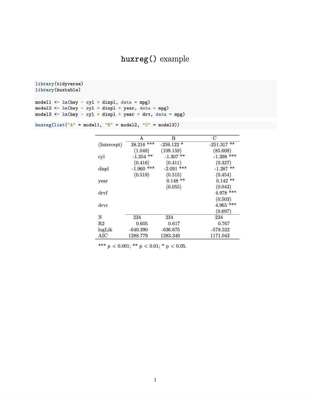
huxtable PDF
---
title: "`huxreg()` example"
output:
  pdf_document: default
---

```{r warning=FALSE, message=FALSE}
library(tidyverse)
library(huxtable)

model1 <- lm(hwy ~ cyl + displ, data = mpg)
model2 <- lm(hwy ~ cyl + displ + year, data = mpg)
model3 <- lm(hwy ~ cyl + displ + year + drv, data = mpg)
```

```{r}
huxreg(list("A" = model1, "B" = model2, "C" = model3))
```
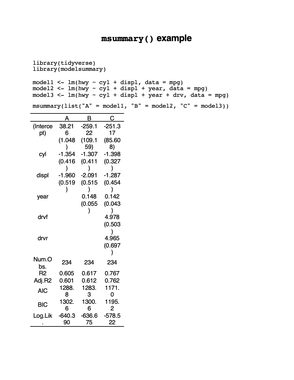
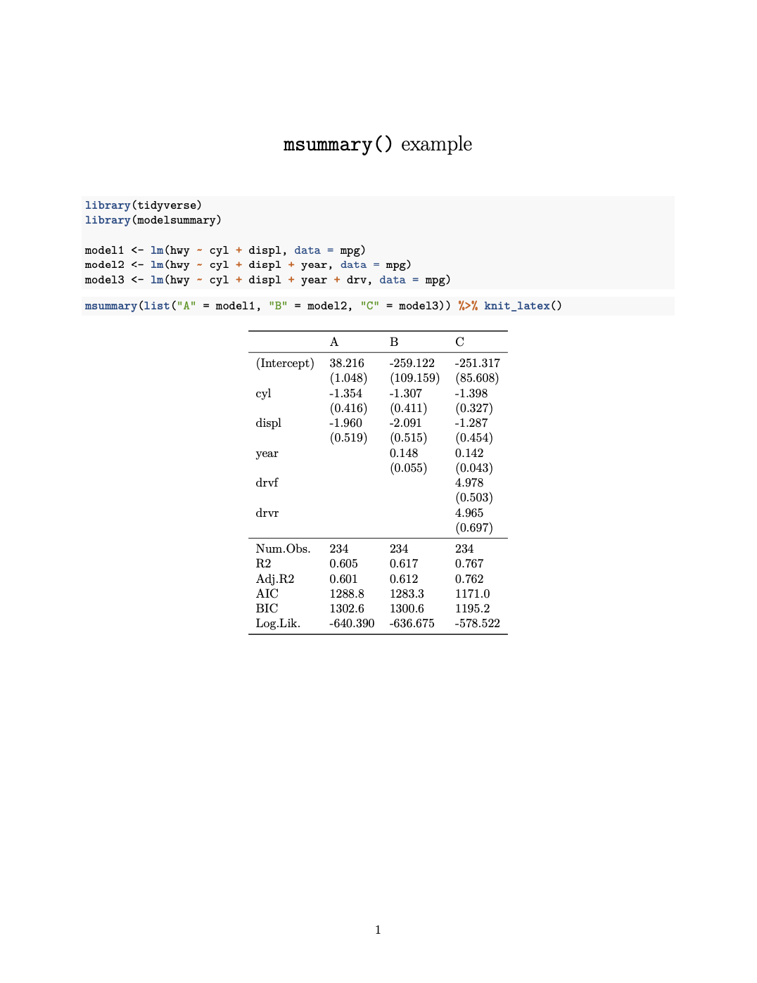
modelsummary PDF
---
title: "`msummary()` example"
output:
  pdf_document: default
header-includes:
- \usepackage{caption}
- \usepackage{longtable}
- \usepackage{booktabs}
---

```{r warning=FALSE, message=FALSE}
library(tidyverse)
library(modelsummary)

model1 <- lm(hwy ~ cyl + displ, data = mpg)
model2 <- lm(hwy ~ cyl + displ + year, data = mpg)
model3 <- lm(hwy ~ cyl + displ + year + drv, data = mpg)
```

```{r}
msummary(list("A" = model1, "B" = model2, "C" = model3)) %>% knit_latex()
```
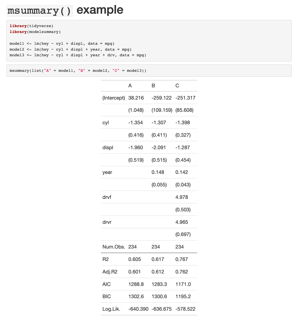
modelsummary HTML
---
title: "`msummary()` example"
output:
  html_document: default
---

```{r warning=FALSE, message=FALSE}
library(tidyverse)
library(modelsummary)

model1 <- lm(hwy ~ cyl + displ, data = mpg)
model2 <- lm(hwy ~ cyl + displ + year, data = mpg)
model3 <- lm(hwy ~ cyl + displ + year + drv, data = mpg)
```

```{r}
msummary(list("A" = model1, "B" = model2, "C" = model3))
```
modelsummary RTF
---
title: "`msummary()` example"
output:
  rtf_document: default
---

```{r warning=FALSE, message=FALSE}
library(tidyverse)
library(modelsummary)

model1 <- lm(hwy ~ cyl + displ, data = mpg)
model2 <- lm(hwy ~ cyl + displ + year, data = mpg)
model3 <- lm(hwy ~ cyl + displ + year + drv, data = mpg)
```

```{r}
msummary(list("A" = model1, "B" = model2, "C" = model3))
```